|
|
|


Hydrological Theory
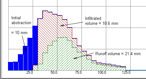
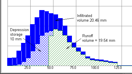
The significance of the components of rainfall loss is illustrated in Figures 7-14 and 7-15. For this comparison the storm used is a 2nd quartile Huff distribution with a total depth of 50 mm over a period of 120 minutes. The rainfall abstractions have been modelled using the SCS Curve Number method with CN = 88.
Figure 7-14 – Rainfall loss components with Ia = 10 mm, Yd = 0.0 Fig 7-14 above shows the normal application of the SCS method in which an initial abstraction Ia = 10 mm has been applied. It is clear that this is a first demand on the storm hyetograph. The remaining 40 mm of rainfall is split into an infiltrated volume of 18.6 mm leaving 21.4 mm of direct runoff.
Figure 7-15 – Rainfall loss components with Ia = 0.0 and Yd = 10.0 mm. Fig 7-15 shows an unusual application of the SCS method developed by means of some of the options in MIDUSS. In this case the initial abstraction is zero so that an infiltration volume of 20.46 mm is the first demand on the storm hyetograph. The remaining 29.54 mm of rainfall is divided between 19.54 mm of direct runoff and 10 mm which is detained as surface depression storage. Note the difference in volume, peak intensity and shape of the direct runoff component. This would certainly be reflected in the resulting overland flow hydrograph. In this example the differences have been exaggerated by using a relatively large depth for Ia or yd. You will find it instructive to recreate this experiment using the Horton method to model the infiltration process or with smaller values of Ia and yd.
|
|||
|
|
|||
|
(c) Copyright 1984-2023 Alan A. Smith Inc. |
|
|